Read the article
here.Jack is a Machine Learning Engineer working on WindBorne AI DA and related WeatherMesh improvements. His primary focus is on improving WindBorne AI DA, though he also has a soft spot for tropical cyclone prediction. Jack had a lot of fun producing Manim visualizations for this post
WindBorne has developed an AI data assimilation (DA) system that officially closes the loop on utilizing our Global Sounding Balloon (GSB) observations to improve forecasts and generate more accurate initial weather conditions. Comparisons to ECMWF’s physics-based DA system show that WindBorne AI DA is 3.5% more accurate at a lead time of 12 hours for the representative variable geopotential height at a pressure level of 500 hPa. To the best of our knowledge, this is the first time an AI-powered DA system is able to obtain lower RMSE scores than ECMWF's DA system, which is widely regarded as the leading standard in assimilation performance. These initial condition improvements, attributed to WindBorne AI DA, allows future iterations of WeatherMesh to continue to improve on record-breaking forecasts and unlock the power of WindBorne Atlas.

Background on DA
To forecast the weather, meteorologists use two key ingredients: initial conditions and a weather model. Initial conditions represent the state of the atmosphere right now, and the weather model forecasts how that weather state will evolve into a new, future, weather state.
Developing accurate weather models that balance low error, high resolution, and efficient computation is critical to weather forecasting. After all, it’s doing the forecasting! However, having accurate initial conditions to start the model is just as important, if not more so, than the predictive power of the model. If we start with an incorrect initial weather state, that initial error will propagate throughout the forecast, ultimately reducing downstream forecast accuracy even if our model is a perfect forecaster! So how do we make sure we have the most accurate set of initial conditions possible? Enter DA.
The DA process typically starts with a noisy weather state called “the background,” which is an old weather state from a previous DA forecast. DA then updates this stale weather state with fresh observations such as those from radiosondes, satellites, and ground weather stations across the globe.
Like model development, building an accurate DA system presents significant challenges: our observations are weird. Whether it be that observations have different noise characteristics, that they may have incomplete global coverage, represent different locations or times, or simply measure different physical variables, we run the gambit when it comes to our observations. Handling these discrepancies between observation types, accounting for deeply nested correlations between observation types, and learning to deal with noisy and uncertain observations is AI’s bread and butter, specifically when leveraging transformers with a lot of data. We firmly believe AI is the definitive next step in DA, and we’re excited to share the results and techniques from our first DA system.
Incoming Observations
Data assimilation lives and dies by the quality of its observations. Getting those observations, however, is far from straightforward. Most DA systems today heavily rely on remote sensing instruments, such as satellite readings, which measure observations from space. These methods offer broad coverage and high volume, but the data is indirect and often noisy.
The kind of observations DA really needs are in-situ observations. These measurements are taken from within the atmosphere itself and offer our weather model a direct view on atmospheric conditions. WindBorne GSBs provide exactly that type of observation, and with WindBorne Atlas well under way, our balloon observations are nearing global coverage. Here’s a quick comparison between WindBorne GSB observations and a satellite reading we use in our AI DA process, AMSU-A satellite readings.

WindBorne GSBs measure temperature, humidity, pressure, and wind speed. GSBs make up Atlas, a constellation of sensors providing constant global weather readings for our Earth. As Atlas grows, the number of high-quality data points we’ll receive will continue to grow, ultimately improving assimilation quality and aligning our initial conditions with reality.

In contrast, the Advanced Microwave Sounding Unit (AMSU-A) satellite remotely monitors the amount of solar radiation being transmitted back from different layers in the atmosphere. This measurement indirectly tells us about the atmosphere’s temperature characteristics, but it's less precise and with higher error. Thus, while AMSU-A is able to take measurements across larger regions, collecting thousands of observations around the globe, each reading only weakly informs our model on the current weather state.
Even though each observation measures the atmosphere differently, together they aim to define the current state of our atmosphere. We can think of DA as the manager of these observations; it is tasked with understanding the physics and purpose of each observation type and leveraging those strengths to produce an accurate weather state.
Our Model
We approach AI DA by leveraging two distinct model phases: an encoding phase and an assimilation phase.
The goal of the encoding phase is to take observations of particular types and, well, encode them into a latent space. A similar encoding step happens for the supplied background weather state, which is encoded into a background latent space. This encoding phase thus generates some amount of distinct latent spaces1 which aim to each represent an observation, allowing us to take in an arbitrary number of observation types. This encoding phase learns to understand what each observation type is measuring and to pick up on some of the nuances within that particular observation type.
We then pass the list of generated latent spaces to the assimilation phase. The assimilation phase takes each of these latent spaces and uses them to imbue the background latent space with observations. The model picks up on correlations between observations and correlations between the background to ultimately make its decision on how to update the latent space.
Encoding Phase
To get more granular with our implementation of the encoding phase, let’s visualize how data flows from observations to the latent space.

Here we have our inputted observations of shape (N, Ch) where N is the total number of observations and Ch is the number of channels. These channels represent data associated with each observation. For instance, in the case of WindBorne balloon data, one channel might represent temperature and another channel might represent pressure.
Our goal is to take these observations and inject them into a latent space so we can later assimilate them to create a weather state. Our latent space is of shape (B, Nvert, D, C) where B is batch size, Nvert is the number of vertices of the underlying HEALPix mesh we use, D is the depth (number of vertical pressure levels), and C is the latent dimension.

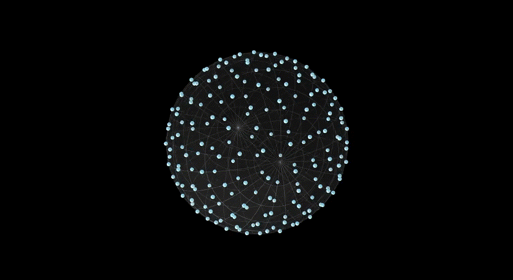
We’ve visualized our HEALPix integration here. This animation demonstrates how we create a HEALPix mesh for every pressure level we care about. For the purpose of this post, we will assume we’re working on one particular pressure level, though in reality we need all of these pressure levels acting in unison since we want them to communicate with one another.

This animation demonstrates that each of these points on the HEALPix mesh is actually a vector of size C. If we have two observations at slightly different locations, we need to find some effective way to encode both of those observations. Yet, we don’t have high enough resolution to encode each separately, therefore, we resort to regions. Each point then represents a local region on the Earth and thus both of these observations get assigned to that point’s embedding which is of size C.

With our observations at the ready and our latent space visualized, we can begin imbuing our latent space with observations. To do so, we first must transform our observations into tokens to take advantage of transformers. With our generated tokens representing our observations, we then leverage cross attention to not just inject our observations into our latent vector, but to allow our latent vector to inform us on how we should go about this injection. We need that two way street to properly take advantage of the fact that multiple observations may be encoded to the same latent vector. This actually comes up quite often considering how our latent space has a limited resolution.
Assimilation Phase

The assimilation phase receives these updated latent spaces from the encoding phase and is tasked with combining them all together into a weather state so we can start our record-breaking forecasting. This is where the bulk of our actual AI DA processing happens, and we approach it by leveraging three distinct transformer elements to give the model just enough inductive bias to properly decide how to combine our observations.
The first transformer allows every observation type to directly communicate with the background without the pollution of other observations. This stage is a one way road between each observation’s latent space and the background they will later be assimilated into.
The second transformer stage is arguably the most important. It takes every observational latent space, along with the background, and updates the background using our observations. This is where our DA happens! We perform this attention across all observations and all relevant pressure levels, though we force each assimilation to occur at a specific location.
Finally, the third transformer stage takes our updated background, and allows observations at different locations to communicate amongst themselves. This effectively counteracts any negative side effects we may incur by forcing assimilation across location as mentioned in the second transformer stage. This then produces our observation-imbued background, and we’re ready to forecast.
Results
To the best of our knowledge, this is the first time an AI-powered data assimilation system is able to obtain lower RMSE scores compared to a control model that uses ECMWF’s physics based data assimilation system. ECMWF’s physics based DA is currently widely regarded as the leading standard in assimilation performance. This leap forward helps bridge gaps in downstream forecasting power as we’re now able to enrich our WeatherMesh model with high quality data as it comes in. Considering the increase in processing speed AI unlocks, these global updates can occur within remarkably fast time intervals.

To form our results, we start with our WM-4 forecasting model. For the control, we stitch in ECMWF’s physics based DA system by inputting HRES at the forecast initialization time. HRES leverages observations from an assimilation window going three hours before the forecast initialization time to three hours ahead, a total window of six hours.
For our actual model, we of course stitch in our AI DA process but instead of using HRES at the forecast initialization time, we input HRES that is six hours old along with all observations from three hours before the initialization time to three hours after. If our DA model can effectively leverage these observations and create an initial condition for the initialization time of our forecast that is better than HRES (and thus ECMWF’s data assimilation system), our forecaster will be better suited for forecasting and we’ll see that through lower RMSE.
An important constant in this evaluation is that our underlying WM-4 model must remain the same between the control model and our actual model in order to isolate the improvement to the DA system. The results are fair if we consider that WM-4 parameters have been frozen during this analysis, and thus have no reason to prefer WindBorne’s AI DA rather than ECMWF’s; WM-4 only cares about accurate initial conditions. If anything, since WM-4 leverages an HRES finetune stage, the base model may tend to prefer initial conditions that match HRES distributions.

It’s worth noting that our results have discrepancies when you control for forecast initialization time. This underlying performance difference is attributed to ECMWF’s HRES showing stronger assimilation for forecast initialization at hours 0z and 12z.


